Hybrid State:Reducing Time-to-Program and Time-to-Train for Industrial Robotics Using Contrastive Language Models Inside Robotic Control State Machines

Abstract
Industrial tasks change with the part, fixture, sequence and exception. Hybrid State lets a robot adapt these decisions while reusing motion that already works. A System 2 model uses a large language model to decompose a goal into ordered actions, write their scripts and define expected outcomes. A local controller follows the scripted waypoints. A System 1 model checks progress, chooses the next state machine and selects a recovery when a step fails.
Hybrid State targets an 86% reduction in combined programming and training time across tasks. During initial task trials, models make decisions within the state machine and learn from the outcomes. An engineer or operator can then lock in successful behavior as fixed waypoints, a learned model, or a combination of both. This lets early trials establish a working control strategy, shortening the process of programming and tuning each step by hand.
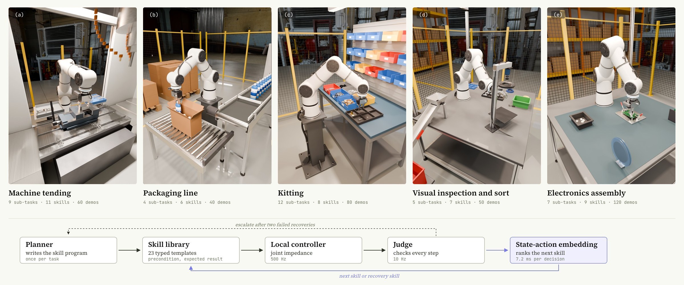
Figure 1. Hybrid State in five simulated industrial cells. Top: (a) machine tending, (b) packaging line, (c) kitting, (d) visual inspection and sort and (e) electronics assembly, each with its number of sub-tasks, skills used and human demonstrations. Bottom: the run-time loop. The planner writes the skill program once per task. The local controller runs each skill at 500 Hz, and the judge checks it at 10 Hz. The state-action embedding ranks the next skill or recovery in a median of 7.2 ms. After two failed recoveries, the task returns to the planner.
1 Introduction
A typical robot cell in a factory runs a program written by an integrator. The program moves through fixed poses, with small offsets from a vision system. It is fast and predictable while every part, fixture and light matches the setup day. When something drifts, the program has no notion of what went wrong. It either stops and waits for an operator or carries on and makes a bad part. Field surveys of automated cells attribute most unexpected stops to such exceptions, not to hardware faults [8].
Learned policies promise to absorb this variation. A visuomotor policy maps camera images directly to arm motion, and it can be trained to cope with shifted parts and changed lighting [4]. Two costs follow. First, the whole task lives in one network, so a new part or a new sequence usually means new demonstrations and retraining. Second, the policy has no explicit record of task progress. Without an explicit step record, a slipped grasp must be inferred from the policy’s visual history.
Hybrid State keeps the structure of a cell program and learns only the decisions that change. The planner, a general-purpose language model, writes a task as an ordered list of skills. A skill is a short, typed motion program such as grasp(billet, top) or place(billet, vise), with a stated precondition and an expected result. The local controller executes a skill at control rate. A judge watches the cameras while each skill runs and decides whether the step succeeded, is still in progress, or failed. When a step fails, the judge picks a recovery skill from a short menu. The choice of the next skill or recovery is made by a learned state-action embedding. It maps the current state and every candidate action into one vector space and ranks the candidates by similarity. Figure 1 shows this loop and the five cells we evaluate it in.
This split matters for three practical reasons. Most decisions inside a task repeat, so the action side of the embedding can be cached and a decision costs a few milliseconds. A change to the task touches the planner's program and a few skill parameters, not a monolithic network. And because every step has an explicit expected result, failures are visible and recoverable rather than silent.
We make four contributions:
- A control stack that separates slow planning, fast skill execution and per-step judgment. Failed steps trigger recovery, and failed recoveries return to the planner (Section 3).
- A contrastive state-action embedding that serves next-skill and recovery decisions with cached action vectors. Its median decision time in our tasks is 7.2 ms (Section 3.3).
- A training recipe that branches simulated episodes from saved states to produce matched successes and failures. These failed alternatives become hard negatives: plausible actions that training learns to reject (Section 3.4).
- An evaluation in five simulated industrial cells against four baselines, with ablations and a failure analysis that names where the approach falls short (Sections 5 to 8).
2 Results
2.1 Success under variation
Table 1 and Figure 2 give the main result. Under held-out variation, Hybrid State completes 83.0% of episodes (95% interval 81.6 to 84.3). It leads the task-specific visuomotor policy by 10.7 points and the scripted program by 31.1 points. The scripted program is the best method in the nominal condition, at 94.5% against 92.0% for Hybrid State. But it loses 42.6 points when the scene changes. Hybrid State loses 9.0.
Table 1. Success rate (%). Nominal and held-out columns pool all five cells. The cell columns are under held-out variation. Bold marks the best value in each column.
| Method | Nominal | Held-out | Tending | Packaging | Kitting | Inspection | Electronics |
|---|---|---|---|---|---|---|---|
| Scripted cell program | 94.5 | 51.9 | 58.3 | 72.5 | 41.0 | 49.7 | 37.8 |
| Fine-tuned generalist policy | 78.2 | 66.3 | 66.0 | 79.3 | 68.8 | 64.8 | 52.7 |
| Task-specific visuomotor policy | 89.4 | 72.3 | 71.2 | 83.0 | 62.7 | 70.3 | 74.3 |
| Planner with skills, no judge | 74.8 | 60.2 | 63.5 | 70.2 | 66.2 | 57.3 | 44.0 |
| Hybrid State (ours) | 92.0 | 83.0 | 88.7 | 91.3 | 84.2 | 79.5 | 71.3 |
The gains are largest where the task has many steps and the scene varies most. In kitting, Hybrid State reaches 84.2% against 62.7% for the task-specific policy. The planner's program keeps track of which parts are already in the tray, and the judge catches wrong picks before the task advances. The planner without a judge reaches only 66.2% in kitting despite the same program. Once one pick goes wrong unnoticed, every later step builds on it.
Electronics assembly is the exception. The task-specific visuomotor policy reaches 74.3% and Hybrid State 71.3%. The insertion itself is one skill. The judge can trigger a retry, but it cannot alter the contact trajectory within the skill. A policy trained end to end on the contact phase learns small corrective motions that our parameterised insert skill does not express. Section 7 returns to this.
2.2 Recovery and cycle time
Hybrid State recovers from 76.4% of injected disturbances (Table 2). The task-specific policy recovers from 38.9% and the planner without a judge from 21.3%. The planner baseline has the same recovery skills, but controller completion can hide the failure that should trigger them. Figure 3 replays one recovery from the episode traced in Figure 10.
Explicit checking costs little time. Hybrid State's cycle time is 1.13 times the scripted program's, against 1.16 for the task-specific policy and 1.56 for the planner baseline. The planner baseline is slow because it waits for a language-model call between every pair of skills.
Swipe sideways to read the figure.
Figure 3. The slip from Figure 10 as a rollout (machine tending, held-out variation, seed 2). The billet slips during the lift at 4.5 s, and the judge rejects the grasp. The embedding selects re-find part and then re-grasp, and the load into the vise is confirmed at 13.5 s. The panel at right shows the four camera views, the current skill, the embedding's ranking and the judge's score. The bar at the bottom is the step timeline.
Table 2. Recovery, speed and robustness. Recovery pools 150 disturbance episodes per cell. Cycle time is relative to the scripted program, so lower is faster. Drop is nominal minus held-out success.
| Method | Recovered after a disturbance (%) | Cycle time (× scripted) | Drop under variation (points) |
|---|---|---|---|
| Scripted cell program | 12.5 | 1.00 | 42.6 |
| Fine-tuned generalist policy | 33.1 | 1.56 | 11.9 |
| Task-specific visuomotor policy | 38.9 | 1.16 | 17.1 |
| Planner with skills, no judge | 21.3 | 1.56 | 14.6 |
| Hybrid State (ours) | 76.4 | 1.13 | 9.0 |
2.3 Adapting to a changed part
We test adaptation with two changes: a new billet geometry in machine tending and a new part number in kitting. Each point pools 300 episodes, split equally between the two changed-part tasks. At zero new demonstrations, the skill program is manually updated for the changed part. All methods receive the new task description and part identifier. We fine-tune learned components on the additional demonstrations only. Hybrid State succeeds in 61.0% of episodes, since only the grasp parameters and one expected-result sentence change. With ten demonstrations it reaches 83.3%. The task-specific policy needs a hundred demonstrations to reach 80.3% (Figure 4).
2.4 Decision latency
With cached action vectors, a decision over 64 candidates takes 7.8 ms. Without the cache it takes 66.9 ms, and asking the planner to score the same menu takes 2.3 s, about 296 times as long (Figure 5). Cached latency grows slowly with menu size, reaching 13.1 ms at 256 candidates against 248 ms uncached. Measurements include state encoding and ranking, with inputs resident on the GPU. They exclude image capture, transfer and low-level control. Cached measurements use warm entries. Uncached measurements rebuild all candidate vectors. Menus in our tasks hold between 8 and 64 candidates.
2.5 Scaling with simulated variation
We hold the episode budget fixed and vary how many authored variations it is spread across. Both methods improve as variation grows (Figure 6). Hybrid State rises from 59.0% with one scene to 83.0% with 27, then levels off at 83.4% with 81. The visuomotor policy follows the same shape at a lower level. The plateau shows diminishing returns within this variation set. It does not establish that appearance no longer contributes to errors. Figure 7 plays a sample of held-out episodes across all five cells.
Swipe sideways to read the figure.
Figure 7. Eighteen short held-out episodes across the five cells, nine at a time in a three-by-three grid. Each tile names its cell, the variation it shows and the current skill. A chip marks each episode's outcome, and two episodes end in a recovery.
3 Method
3.1 System overview
Figure 8 shows the run-time loop, and Figure 9 animates it. The System 2 model reasons about the goal, breaks it into ordered actions, writes a script for each action and defines how to recognise its outcome. These programs form the state machine library: reusable actions with explicit transitions, parameters and completion conditions. The local controller executes their waypoints. The System 1 model reads the cameras and robot state, checks progress and ranks the next eligible state machine or recovery. Its response target is under 50 ms, so these decisions can follow the changing scene without waiting for another full planning call. This target concerns model response time, separate from camera capture and the controller cycle. After two failed recoveries on one sub-task, the System 2 model revises the remaining program.
System 2 Model
A large language model decomposes the goal into ordered actions.
Writes each action’s script and defines its expected outcome.
State Machine Library
Action scripts, transitions and expected outcomes
Local Controller
Runs the current skill at 500 Hz
Holds position if a target goes stale
Cameras + Robot State
Overhead view, wrist view, joints, gripper
System 1 Model
Check progress and expected outcomes
Choose the next state machine
Choose a recovery state machine
Responds to the changing scene without waiting for a new plan.
System 2 Model
Reviews the failure and rewrites the remaining actions
Episode Recordings
System 1 Model
Proposes success, failure and recovery labels for review
Embedding Training
Swipe sideways to read the figure.
Figure 9. Figure 8 animated over one machine-tending task, including the data loop between training rounds. The animation is schematic and is not the episode in Figure 10.
3.2 System 1 judgment and recovery
The System 1 model combines outcome judgment with action selection. Its judge checks whether the observed state is consistent with the current skill phase. During execution, it compares the state with a description of expected progress, such as “the billet remains in the gripper during the lift”. At the end, it checks the final expected result, such as “the billet rests against the vise stop”. Both descriptions are encoded like actions, and observations like states, using the embedding of Section 3.3. A learned scale and offset calibrate their similarity. A sigmoid maps this value to a score between zero and one. The calibration is fitted on human-labelled step checks with binary cross-entropy, a loss for success and failure labels. A score above 0.5 at the end confirms completion. During execution, a fall below 0.5 after a score above it triggers recovery. The phase description is part of the state’s sub-task text.
Figure 10 traces one machine-tending episode. The billet slips in the gripper during the lift. The judge’s score falls below the threshold at the marked slip. The embedding ranks re-find part first, then re-grasp, and the step is confirmed at the vise. Without the judge, the controller would have reported the lift as done and carried an empty gripper to the machine. Figure 11 shows the same pattern in the inspection cell.

Swipe sideways to read the figure.
Figure 11. A recovered grasp in the inspection cell. (a) The housing has slipped onto the bench, and the jaw closes on an empty pocket. (b) The judge flags the slip in the overhead view. (c) The re-find part skill locates the housing in the wrist view. (d) The arm grasps it again across its side. (e) The arm carries the housing back over its empty pocket, and the judge confirms the step.
3.3 State-action embedding
The embedding scores how well a candidate action fits the current state. The state s contains the overhead and wrist images, the seven joint angles and the gripper width, the current sub-task and skill phase as text, and the last two judge outcomes. In the inspection cell, it also contains the predicted defect class. An action a is a skill name, its parameters and its precondition text. A frozen pretrained vision-language encoder E turns both into features. Joint values are normalised to their limits and written as numeric text alongside the skill description. Two small learned projection networks (heads), hs for states and ha for actions, project these features into one 256-dimensional space (Equation 1).
Training: fit a shared decision space
Normalize the state representation
Normalize the action representation
Each projected vector is normalised to unit length, so the dot product of a state and an action measures their agreement.
Score the match between state and action
Learn matching pairs in both directions
U is the square matrix of scores between the batch’s matched states and actions. V extends each row of U with up to seven actions that failed from that row’s saved state. Missing entries are masked. The target y selects the matching pair, and CE denotes cross-entropy. The first term trains state-to-action matching with the failed branches. The second uses only the square matrix to train action-to-state matching. Equivalent successful actions are masked out as negatives. The learned scale α controls score separation.
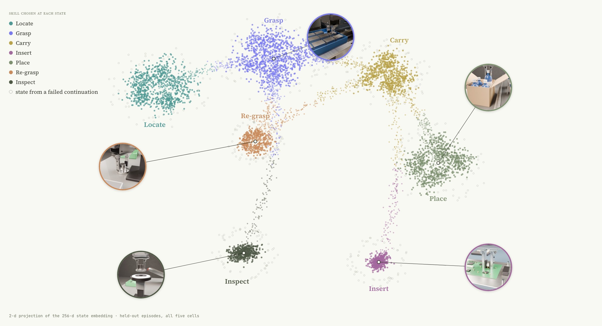
At run time the same model ranks the candidates (Figure 13). The candidate set A contains instantiated skills whose preconditions hold, or the recovery menu after a failure. A template can yield several candidates with different parts, poses or grasp parameters. Because the two heads are separate, action vectors depend only on the action text. The cache key includes the skill, bound parameters and precondition text. Entries are reused while this text stays unchanged. A changed perception estimate or program invalidates the affected entries. With a warm cache, each decision encodes one new state and takes one small matrix product. The median decision in our tasks takes 7.2 ms, of which 5.4 ms is the state encoder. Figure 14 projects held-out decision states into two dimensions. The projection illustrates grouping by the selected skill. Cell identity is not encoded in this view, so the plot does not by itself show how cells mix.
Serving: encode the new state, reuse the actions
Rank the eligible actions
The controller runs the highest-ranked candidate. If the top two candidate probabilities differ by less than 0.05, the decision is logged for review but not blocked.
Swipe sideways to read the figure.
Figure 14. A two-dimensional projection of the 256-dimensional state embedding for decision states from held-out episodes in all five cells. Each filled point is a state, coloured by the skill the embedding ranked first. Hollow rings show states observed in failed continuations. The failed actions that produced them supply the hard-negative examples of Section 3.4. Circular insets show a representative state for five skills. Paths between clusters follow common transitions, such as grasp to carry and carry to place. The projection is for illustration only, and distances in it do not equal embedding similarities.
3.4 Training data and branched hard negatives
A successful demonstration shows one workable path, but it rarely explains what to do when that path fails. Programmatic waypoints let the robot repeat known motions across simulated task variations and collect new examples without a person demonstrating every attempt. Branching makes these examples more informative: alternative actions start from the same observation, so the model can learn which choice caused success or failure. Failed but plausible choices are hard negatives. They teach the model to distinguish close alternatives, improving state-machine selection and recovery while concentrating training on decisions the robot still gets wrong.
Each cell starts from 40 to 120 human demonstrations, recorded by teleoperation in simulation and segmented into skills. We repeatedly replay demonstration skill programs across 27 authored variations per cell, varying initial part poses within each layout. Rollouts continue to the per-cell episode budgets in Table 3. This produces 260,000 episodes in total across the five cells (Table 3). The judge is first trained on human-labelled checks from the demonstrations. It then proposes success and failure labels for replayed steps. Recovery labels come from the identity of the executed skill. Labels near the threshold go to a human reviewer. About 3% of steps needed review.
Random negatives are easy. A place skill is rarely a plausible answer when the gripper is empty. The useful negatives are actions that look right but fail. We create them by branching (Figure 15). At each sampled decision point in a successful episode, we save the simulator state and run up to seven alternative eligible skills from it. These continuations are additional training pairs, not full episodes in Table 3. Human-reviewed judge outcomes determine which alternatives failed. The final task score alone reads simulator ground truth. Branches from one saved state always stay in the same data split, so evaluation never sees a near-copy of a training state.
 Shared starting evidence
4 Simulated Cells
We evaluate in five industrial cells built for this study [12]. Each cell uses the same 7-axis industrial arm on a fixed pedestal. Every cell uses the same parallel gripper. Every cell has a fixed overhead camera and a wrist camera. These are the only two views the policy and the judge receive. The inspection cell adds a station camera that only the inspect skill reads. Two further views, from the side and front, are recorded for analysis only. Table 3 summarises the cell tasks.
Table 3. The five cells. Sub-tasks are steps in the planner's program for one task. Skills used counts the distinct templates the program draws on, including recovery skills.
| Cell | Task | Sub-tasks | Skills used | Human demos | Sim episodes |
|---|---|---|---|---|---|
| Machine tending | Load a billet into a vise, close the door, start the cycle, unload the finished part to a tray. | 9 | 11 | 60 | 48,000 |
| Packaging line | Pick the front bottle from an indexing infeed belt and place it upright in the next empty slot of a 3 by 4 case. | 4 | 6 | 40 | 36,000 |
| Kitting | Fill a kit tray from mixed-part bins in the order the work order lists. | 12 | 8 | 80 | 64,000 |
| Visual inspection and sort | Present each part beneath the ring light and station camera, then place it on the pass tray or into the reject chute. | 5 | 7 | 50 | 40,000 |
| Electronics assembly | Pick a board-to-board connector and seat it on a fixtured circuit board. | 7 | 9 | 120 | 72,000 |
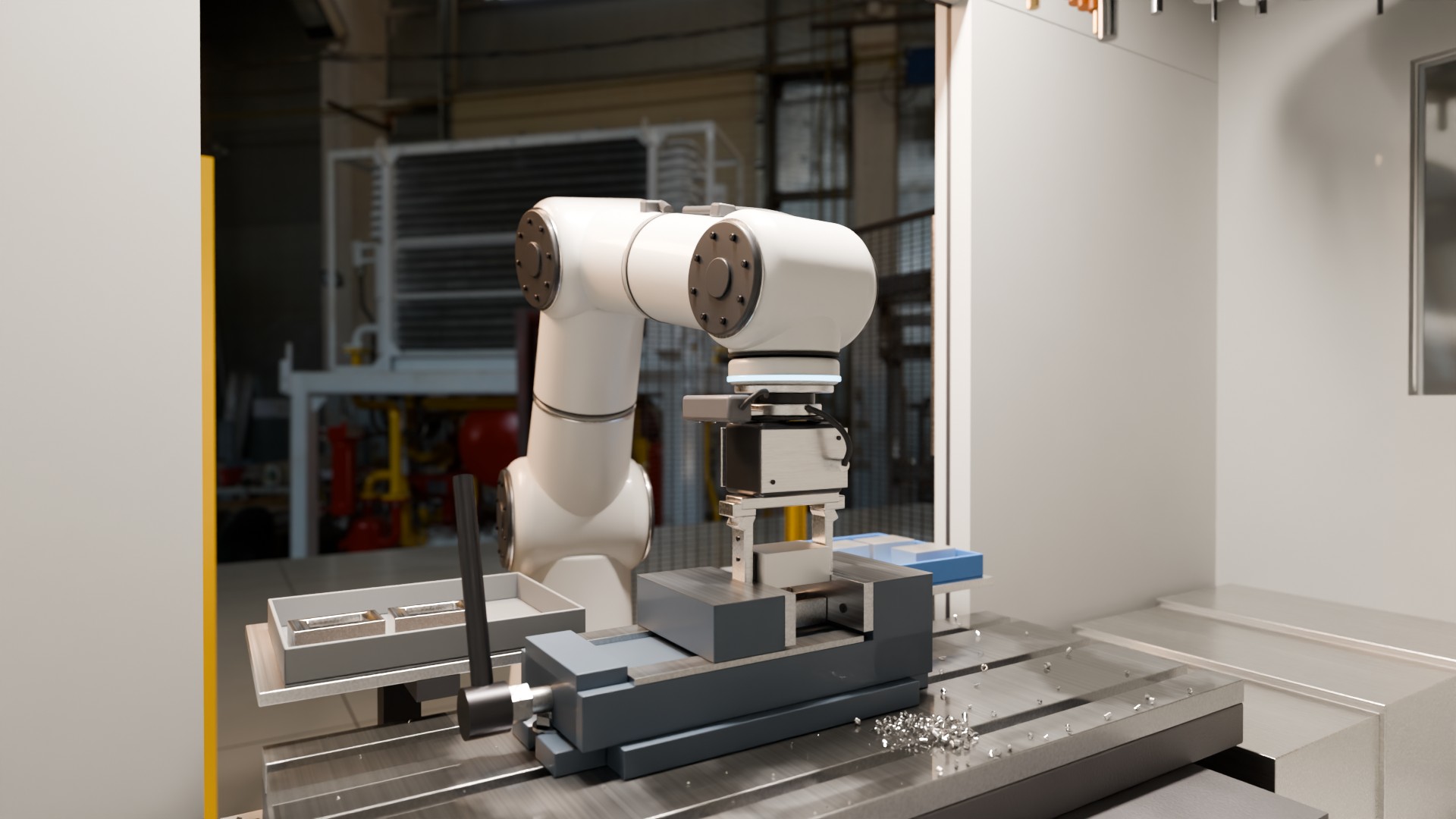
Machine tending. The arm takes a billet from a raw-stock tray, loads it into the vise of a milling machine, closes the door and starts the cycle. When the cycle ends it unloads the finished part to a second tray (Figure 16). Chips on the machine table make the vise area visually busy. Hybrid State completes a successful tending cycle in a median of 45.7 s. Figure 18 plays one such episode from start to finish.
Figure 16. The machine-tending cell, seen from inside the machine. The arm reaches through the open door and lowers an aluminium billet, held by its two ends, into the open vise. Chips lie on the machine table. Raw billets wait in the blue tray on the right, and finished parts go to the grey tray on the left.
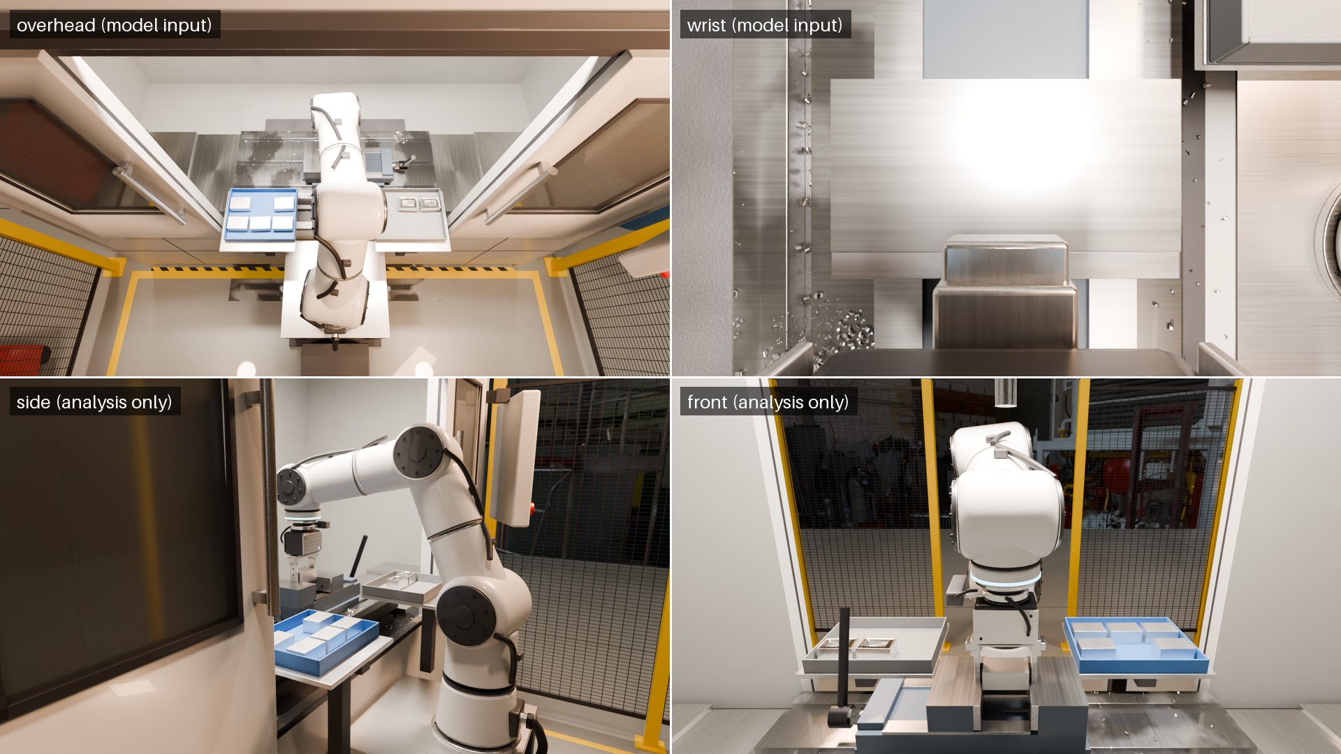
Figure 17. One moment in the machine-tending cell from four cameras. The overhead and wrist views (top) are the model's inputs. The side and front views (bottom) are for analysis only. The wrist view looks down at the billet between the vise jaws.
Swipe sideways to read the figure.
Figure 18. One complete machine-tending episode in the nominal cell (seed 0), played at 1.8 times real time. The arm grasps a billet, loads and clamps it in the vise, and the door closes for the cut. It then unloads the finished part and places it in the tray. All nine sub-tasks are confirmed by the judge, and the episode ends at 45.7 s of simulated time. The overlay shows the current skill, the embedding's ranking, the judge's score and each step's verdict.
Packaging line. Bottles queue on an infeed belt that indexes one pitch at a time. The arm takes the front bottle by its cap and places it upright in the next empty slot of a three-by-four case on a roller table (Figure 19). The task is short but timing-sensitive, since each grasp must finish between index moves.
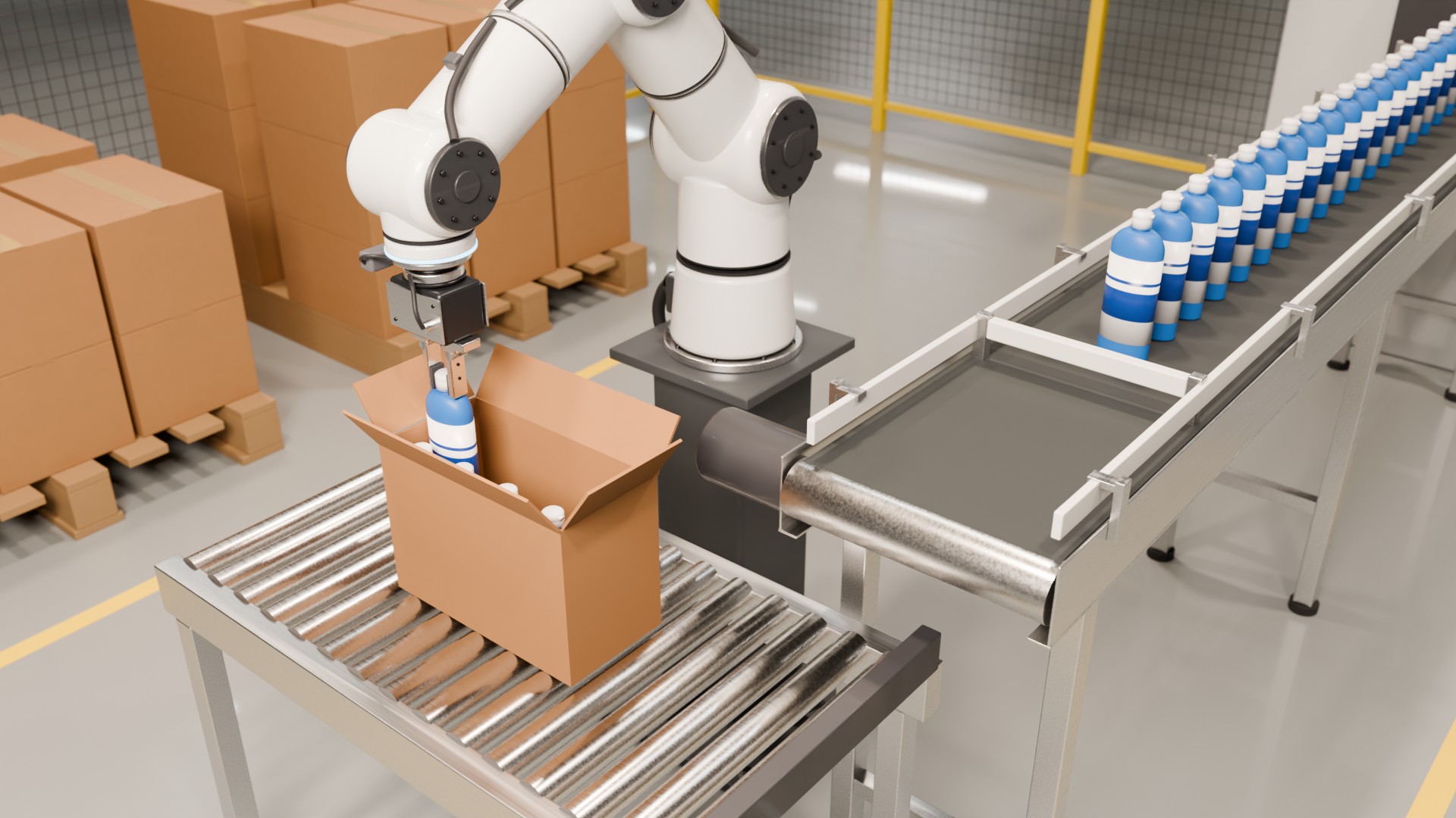
Figure 19. The packaging cell. The arm lowers a bottle, gripped by its cap, into an open case on a roller table. More bottles queue on the infeed belt, and pallets of sealed cases stand behind the cell.
Figure 20. One packing cycle. The arm takes the front bottle from the infeed belt, the queue indexes one pitch toward the station, and the arm places the bottle in the case.
Kitting. A work order lists six parts. The arm picks each from one of six mixed bins and places it in the matching pocket of a kit tray. Bins hold look-alike parts, so the main difficulty is finding the right part, not grasping it.
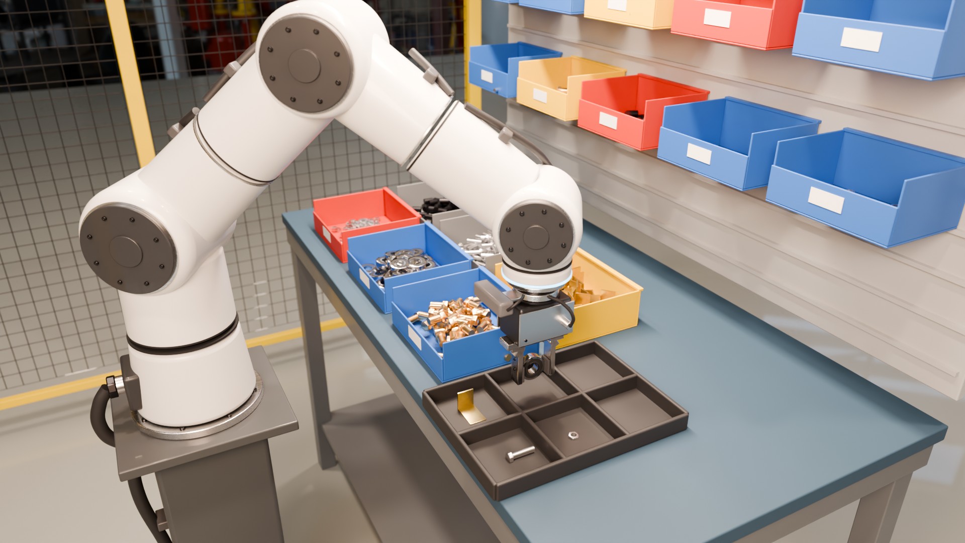
Figure 21. The kitting cell. Three of the tray's six pockets already hold one bolt, one nut and one bracket, and the arm places the bearing in a fourth. Six bins of mixed hardware sit on the bench, and more bins hang on the panel behind.
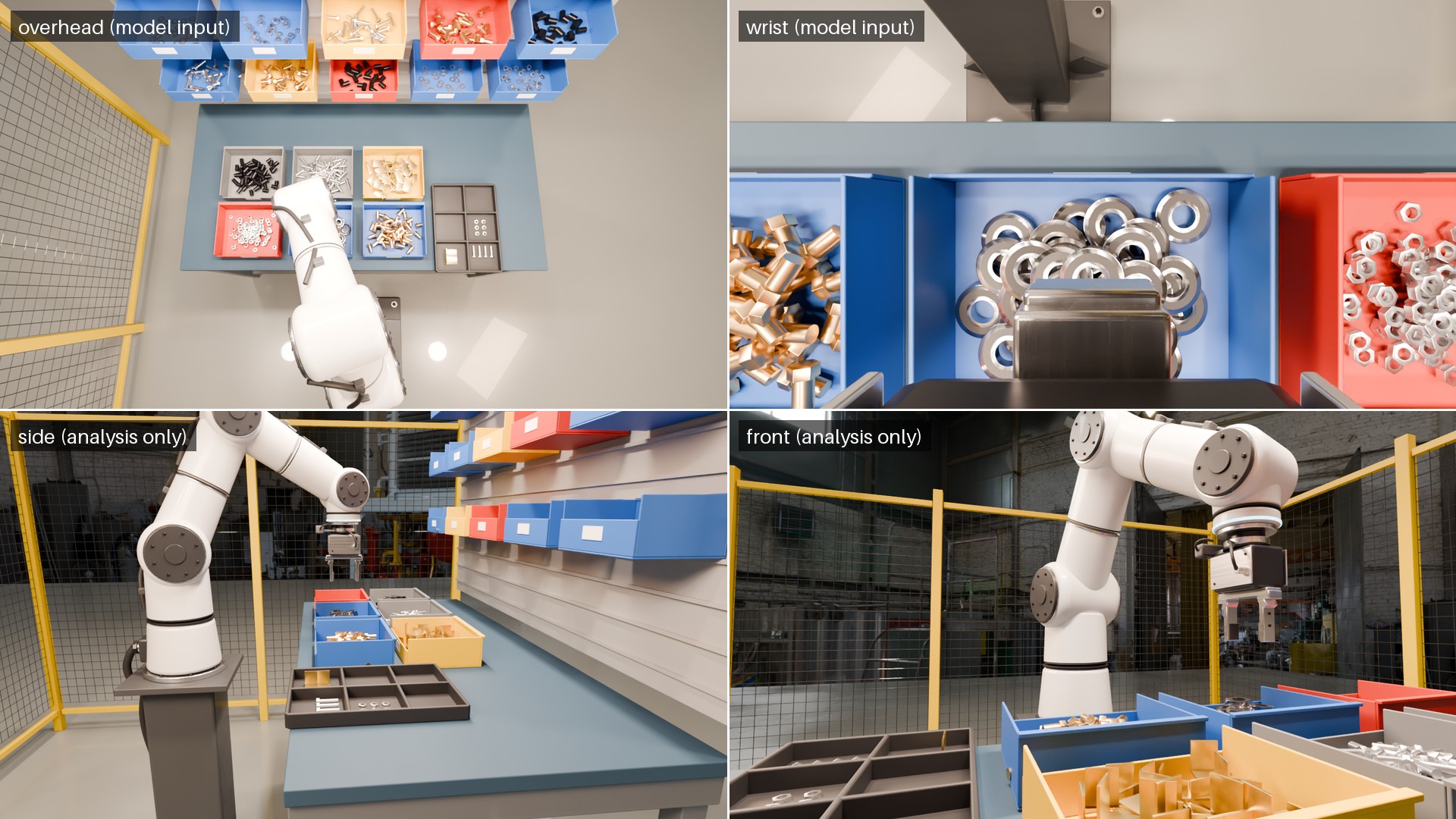
Figure 22. One kitting moment from four cameras, with the arm over the bearing bin and its fingers open. In the wrist view (top right), bearings of two sizes, 47 mm and 40 mm, lie mixed in one bin. Look-alike parts like these are the largest cause of kitting failures, 38 of 95 (Section 7).
Visual inspection and sort. The arm takes a machined housing from an infeed tray and holds it under a ring light in two poses. A downward station camera above the light images it (Figure 23). It then places the part on a pass tray or drops it into a reject chute. The defect label comes from the scene definition and is never shown to the policy. A shared inspection routine reads the station image and returns a predicted defect class. All methods receive this prediction, and no method receives the true label. The judge verifies presentation and sorting from the overhead and wrist views against that prediction, so a classification error can also become a false completion.
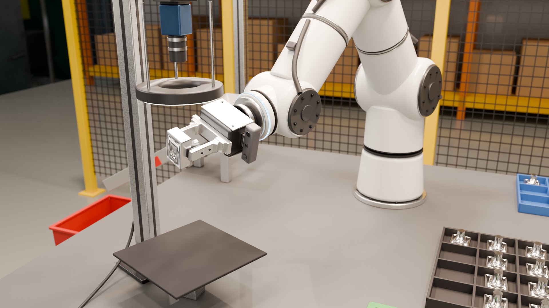
Figure 23. The inspection cell. The arm holds a machined housing in its parallel gripper beneath the ring light and the downward station camera. A reject chute beside the station carries rejected parts down to the red bin on the left. The infeed tray of unsorted housings is at the lower right, and the blue pass tray is at the right edge.
Figure 24. An inspection sequence. The arm lifts a housing from the infeed tray and rotates it beneath the ring light. The sorting step is not shown. The bench carries clutter from one of the training variations.
Electronics assembly. The arm picks a board-to-board connector from a feeder and seats it on a circuit board held in a fixture on an anti-static mat. Seating needs about 2 mm of travel with under 0.3 mm of lateral error (Figure 25). It is the most contact-rich task in the set.
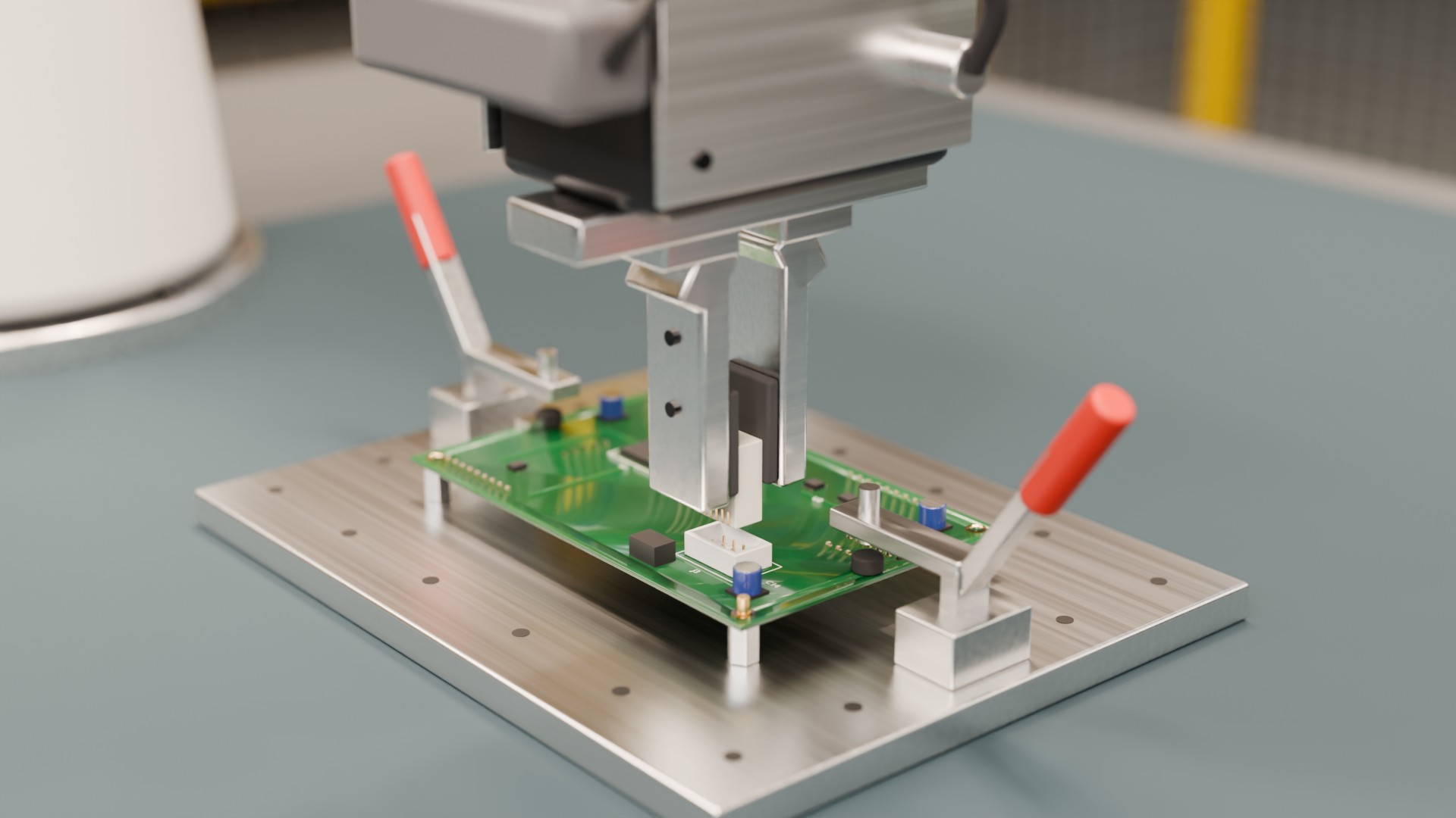
Figure 25. The electronics cell. The gripper holds a board-to-board connector between its pads, just above its receptacle. Two toggle clamps hold the circuit board in an aluminium fixture on an anti-static mat.
Figure 26. The insertion move at close range. The arm aligns the connector over its receptacle, presses it home, releases it and withdraws, leaving the connector seated on the board.
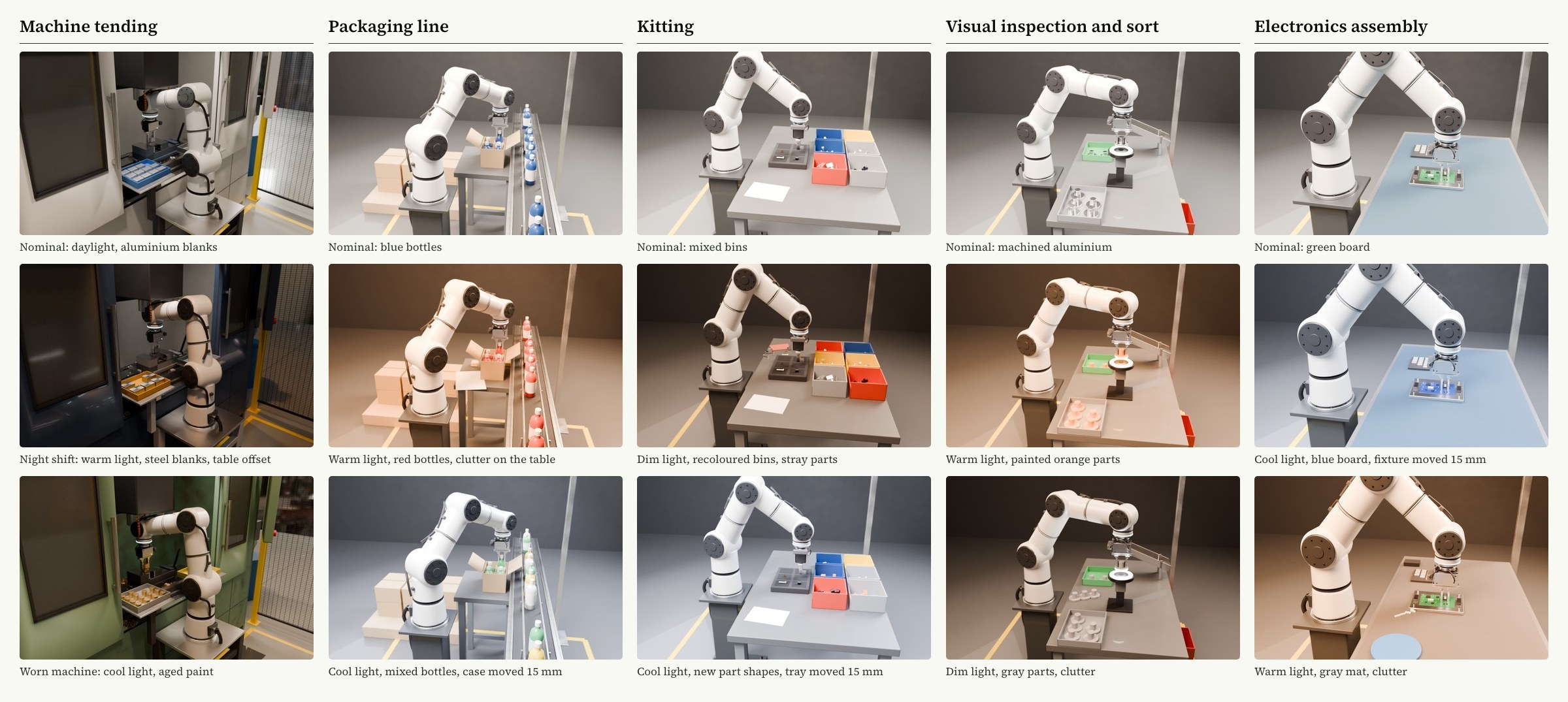
Variation. Each cell has 27 authored training variations and a separate set of held-out variations used only for evaluation. Variations change four things: lighting, part colour and geometry, fixture position (offsets up to 15 mm), and clutter in the workspace. Figure 27 shows three variations of each cell, and Figure 28 shows the inspection cell under nine. Held-out variations combine these factors in ways not seen in training and include part geometries outside the training set.
Swipe sideways to read the figure.
Figure 27. Fifteen of the authored scene variations, three per cell. The top row shows each cell in its nominal configuration. The two lower rows change lighting, part colour and geometry, fixture position and clutter, as labelled under each panel. Panels use simplified versions of the cells shown in Section 4.
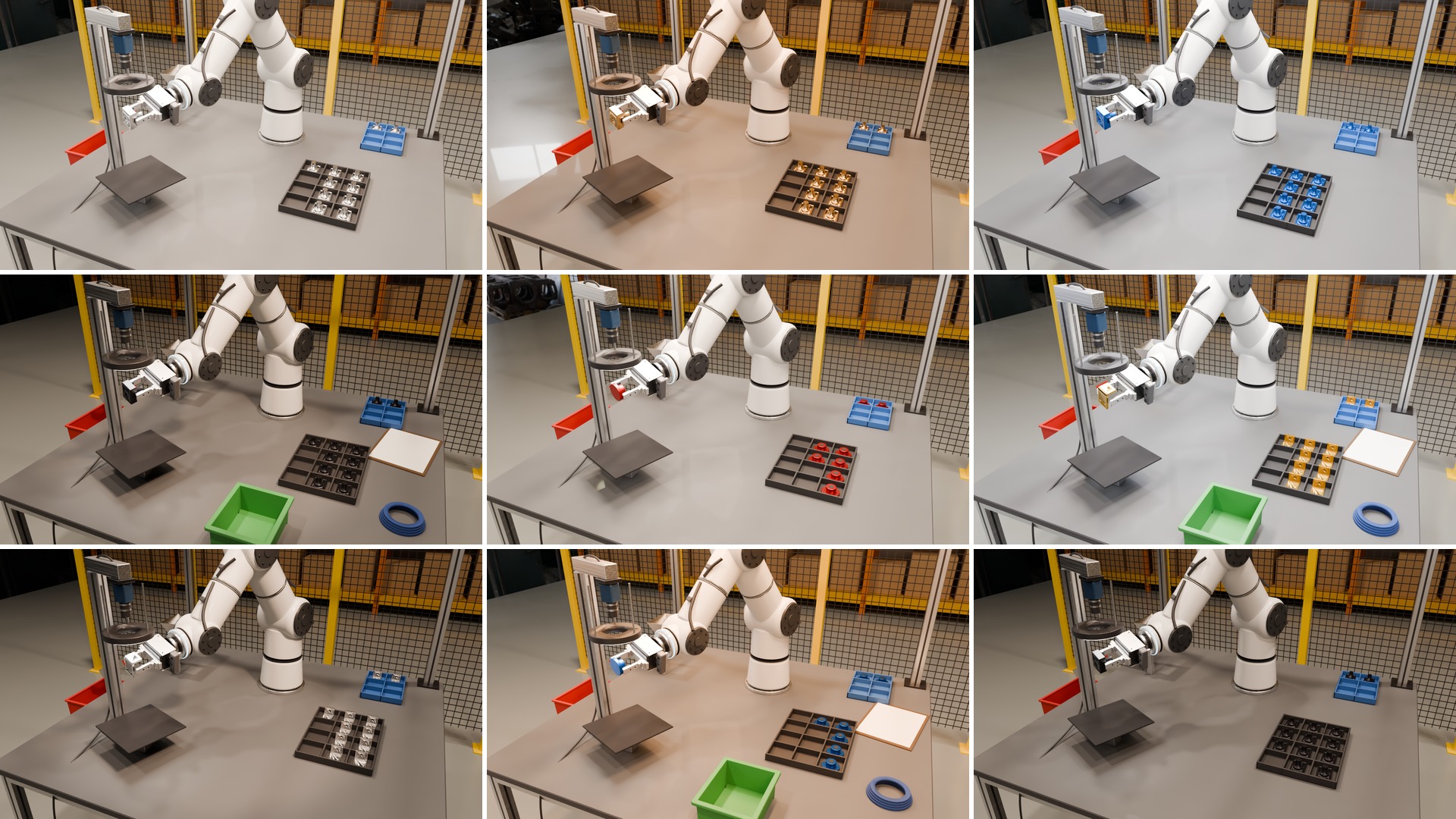
Figure 28. The inspection cell under nine authored variations, read left to right and top to bottom. (1) Nominal. (2) Warm light, brass housings. (3) Cool light, blue parts, tray moved. (4) Spot light, black parts, worn bench, clutter. (5) Red flanges. (6) Cool light, gold brackets, station moved, clutter. (7) Spot light, raw brackets, tray moved. (8) Warm light, blue flanges, clutter. (9) Dim light, black housings, worn bench, tray and station moved. The task is the same in every panel.
5 Experiments
5.1 Setup
All experiments run in simulation. For each cell and method we use 3 evaluation seeds and run 200 evaluation episodes per seed. That gives 600 episodes per cell and method in each condition, and 30,000 episodes in the main evaluation. Disturbance, adaptation and ablation trials are additional. Learned methods have a separately trained model for each seed. Scripted programs are fixed. The nominal condition uses the training variations with fresh initial states. The held-out condition uses the unseen variations described in Section 4. We report pooled success rates with 95% Wilson intervals. Differences and ratios are computed before displayed values are rounded. These intervals describe pooled episode outcomes, not uncertainty across training seeds. Shared layouts can correlate episodes, so the intervals are descriptive rather than evidence of statistical significance.
5.2 Baselines
All methods receive the same overhead and wrist images, the same robot state and the same human demonstrations. The learned baselines also train on the same 260,000 complete simulated episodes. In the inspection cell, all methods also receive the shared inspection routine's predicted defect class. Hybrid State additionally receives the branched decision pairs. The hard-negative ablation measures this extra supervision. The main comparison does not equalise total training pairs.
- Scripted cell program. A hand-written program in the style of an integrator, with taught waypoints, vision offsets from the overhead camera and a single retry on a failed grasp.
- Fine-tuned generalist policy. A pretrained language-conditioned visuomotor policy [5], fine-tuned per cell on the same data. It receives the task description as text.
- Task-specific visuomotor policy. An action-diffusion policy [4] trained from scratch for each cell. It predicts 16-step chunks of joint targets.
- Planner with skills, no judge. The same planner and skill library as Hybrid State, but each skill is treated as done when the controller reports that it finished. The planner picks the next skill from text and a scene caption, with no learned embedding.
5.3 Metrics
Success is the fraction of episodes that meet the cell's success rule within its time limit (Appendix B). Recovery is the fraction of 150 disturbance episodes per cell in which the task still succeeds. In these, we inject one fault mid-task: a forced grasp slip, a part nudged by 20 to 40 mm, or a one-second occlusion of the wrist camera. Cycle time is the median duration of successful held-out episodes, including recovery and planner calls. Machine tending includes a fixed simulated machining dwell. Because failed episodes are excluded, this metric is not production throughput. We report it relative to the scripted program, averaged across cells by geometric mean. For the judge we report false completion, a failed step confirmed as done, and missed completion, a finished step not confirmed. Both percentages divide the error count by all end-of-skill checks, rather than by failed or finished steps separately. Human review of recorded views supplies the reference labels. Adaptation is success after a part change, against the number of new demonstrations.
6 Ablations
We remove one part of Hybrid State at a time and rerun the held-out evaluation (Table 4, Figure 29). Training in a single nominal scene costs the most, at 24.0 points. Among the parts of the run-time system, the judge matters most. Without it, skills end on the controller's own done signal, success falls by 13.6 points and recovery falls from 76.4% to 24.8%. Keeping the judge but allowing only a retry of the failed skill, with no recovery menu, costs 8.4 points.
Replacing the embedding with the planner for every decision costs 4.8 points and makes cycles 41% longer. The drop is largest in electronics assembly (7.3 points), where delayed decisions coincide with loss of alignment between steps. This ablation changes both decision timing and selection, so it does not isolate latency as the cause. Removing the wrist camera costs 7.0 points overall but 12.8 in electronics, where the overhead view cannot resolve the connector pins. Training without branched hard negatives costs 3.9 points. On held-out decision points it lowers top-1 accuracy, the share of decisions where the right action ranks first, from 91.4% to 84.7%.
Table 4. Ablations under held-out variation, pooled over all cells. Change is relative to the full system.
| Variant | Success (%) | 95% interval | Change (points) | Recovered (%) |
|---|---|---|---|---|
| Full system | 83.0 | 81.6 to 84.3 | 76.4 | |
| No branched hard negatives | 79.1 | 77.6 to 80.5 | −3.9 | 72.1 |
| Planner picks every skill (no embedding) | 78.2 | 76.7 to 79.7 | −4.8 | 71.7 |
| No wrist camera | 76.0 | 74.4 to 77.5 | −7.0 | 66.3 |
| Retry only, no recovery skills | 74.6 | 73.0 to 76.1 | −8.4 | 41.2 |
| No judge (controller done flag) | 69.4 | 67.7 to 71.0 | −13.6 | 24.8 |
| One nominal scene, no variation | 59.0 | 57.3 to 60.8 | −24.0 | 51.2 |
7 Failure Analysis
We labelled the cause of every failed Hybrid State episode under held-out variation by reviewing the four recorded views (Figure 30). Across all cells, grasp and contact errors account for 35% of failures, perception errors for 24% and judge false completions for 17%. The mix differs sharply by cell.
Contact in electronics assembly. Of 172 failed electronics episodes, 101 (59%) are insertion failures: a connector seated at an angle, or pins that stubbed and did not engage. The insert skill follows a fixed search pattern once it touches the board. The task-specific policy instead learned to tilt and rock the connector, a correction the skill cannot express. This difference is consistent with the task-specific policy’s advantage in this cell.
The judge on reflective parts. In the inspection cell, 44 of 123 failures are false completions by the judge. Its false completion rate is 1.8% there, against 0.8% in the other four cells combined (Table 5). Polished parts under the ring light produce specular highlights that hide small defects in the station image. The inspection routine then labels a defective part as good. The judge checks the sort from the overhead and wrist views, which cannot resolve the defect either, so it confirms the wrong outcome. The remaining 25 false completions occurred while presenting the part and were caught by the next skill's precondition.
Look-alike parts in kitting. In kitting, 38 of 95 failures come from picking a similar but wrong part. The judge usually catches these at the tray. When the embedding then picks the same wrong part again, the task runs out of time. We count these as perception failures, the root cause, even though the episode ends at the time limit.
Table 5. Judge errors by cell under held-out variation. A step check is one end-of-skill decision. Both error percentages use all step checks as their denominator. False completion confirms a failed step. Missed completion withholds confirmation from a finished one.
| Cell | Step checks | False completion (%) | Missed completion (%) |
|---|---|---|---|
| Machine tending | 5,940 | 0.7 | 2.4 |
| Packaging line | 2,410 | 0.5 | 2.1 |
| Kitting | 7,070 | 0.6 | 2.6 |
| Visual inspection and sort | 3,816 | 1.8 | 2.6 |
| Electronics assembly | 3,424 | 1.7 | 3.5 |
8 Limitations
All results in this paper come from simulation. The cells are detailed, but contact, friction, cable drag and camera noise are modelled, not measured. Contact-rich tasks such as connector insertion are where simulation is least faithful, so the electronics results are the least certain here. We have not yet run the system on physical hardware.
The skill library is written by hand. A task whose difficulty lies inside a single skill, such as insertion, gains little from planning and judgment, as electronics assembly shows. Learning the inside of such skills, for example with a local visuomotor policy behind the same interface, is the most direct next step.
The judge sees no more than the robot's own cameras. Where those views cannot resolve the outcome, as with small defects on reflective parts, the judge cannot catch the error. An independent signal, such as a force reading or a second inspection angle, would make its checks more trustworthy.
Finally, the planner is an off-the-shelf language model. We did not study how its errors propagate, and the five reported tasks passed a preliminary planner screen. Tasks with an incorrect first program in more than 5% of screening attempts were outside the study. Results are conditional on this screen and do not measure reliability on unrestricted goals.
9 Conclusion
Hybrid State treats an industrial task as a program of checked steps. A slow planner writes the program, a fast controller runs it, and a judge verifies each step. A learned state-action embedding makes the many small decisions in between. In five simulated cells this structure holds up under variation better than scripted programs or end-to-end policies. It recovers from most injected faults and adapts to a new part with a handful of demonstrations. Its weak points are just as clear: contact-rich motion inside a single skill, and a judge limited by the robot's own cameras. Both suggest the same direction. Keep the checked program as the backbone, and put more learning inside the skills and more independent evidence behind the checks.
Citation
@techreport{standardmatter2026hybridstate,
  title       = {Hybrid State: Reducing Time-to-Program and Time-to-Train for Industrial Robotics Using Contrastive Language Models Inside Robotic Control State Machines},
  author      = {Keane, Wes and Sriram, Abhinav},
  institution = {Standard Matter},
  year        = {2026},
  month       = oct
}
References
- Industrial Manipulation Benchmark Consortium. Benchmarking robot cells for machine tending and kitting. Technical Report IMBC-TR-2025-03, 2025.
- Hierarchical Task Planning Working Group. Language models as task planners for robot cells: a survey. Survey series HTP-S-07, 2025.
- Open Skill Library Initiative. Parameterised motion primitives for industrial arms. Technical Report OSLI-TR-2024-11, 2024.
- Open Visuomotor Benchmark. Action diffusion for imitation in manipulation: a reproducibility study. Benchmark report OVB-R4, 2025.
- Generalist Robot Policy Collaboration. Fine-tuning language-conditioned generalist policies on new embodiments. Collaboration report GRPC-2025-02, 2025.
- Contrastive Representation Workshop. Dual encoders for state-action matching. In Proceedings of the 2024 Workshop on Representation Learning for Control, 2024.
- Simulation at Scale Initiative. Demonstration expansion by replay in randomised scenes. Technical Report SAS-TR-2024-06, 2024.
- Factory Automation Reliability Forum. Exception handling in automated work cells: a field survey. Forum report FARF-12, 2025.
- Success Detection Benchmark. Learned success detectors for long-horizon manipulation. Benchmark report SDB-2025-01, 2025.
- Sim-to-Real Transfer Consortium. How much variation is enough? Scene randomisation for transfer. Technical Report S2R-TR-2024-09, 2024.
- Retrieval for Control Workshop. Embedding caches for low-latency decision serving. In Proceedings of the 2025 Retrieval for Control Workshop, 2025.
- Standard Matter. Hybrid State cell kit: authored industrial cells for robot learning. Technical note SM-TN-2026-04, 2026.
Appendix
A. Hyperparameters and compute
Simulated episodes were generated on 256 simulation workers, with rendering taking 410 GPU-hours. Training the embedding heads and the judge took 96 GPU-hours. Table 6 lists the main settings.
Table 6. Hyperparameters for the embedding, judge and controller.
| Setting | Value |
|---|---|
| Frozen encoder | Pretrained vision-language transformer, 0.4B parameters, 224 px input |
| State input | Overhead and wrist images, 7 joint angles normalised to joint limits and gripper width as numeric text, current skill phase, last two judge outcomes, and the predicted defect class in the inspection cell |
| Action input | Skill name, typed parameters and its precondition text |
| Judge calibration | Affine calibration of state–phase similarity followed by a sigmoid, fitted on human-labelled checks with binary cross-entropy |
| Projection heads | Two-layer projection networks with 1,024 hidden units and 256-dimensional outputs, one each for state and action |
| Batch size | 4,096 state-action pairs |
| Hard negatives | Up to 7 failed branches per saved state |
| Optimizer | AdamW, learning rate 3e-4, weight decay 0.05, cosine decay, 2,000 warm-up steps |
| Training steps | 60,000 |
| Similarity scale | Learned inverse temperature, initialised at 1/0.07 and clipped at 100 |
| Local controller | Joint impedance at 500 Hz, skill targets at 30 Hz |
| Judge rate | 10 Hz while a skill runs, plus one check when it ends |
| Recovery budget | Two failed recovery attempts per sub-task, then escalation to the planner. Successful recovery steps do not consume this budget. |
| Planner | Off-the-shelf language model, no fine-tuning, called once per task and on escalation |
| Variation axes | Lighting, part colour and geometry, fixture offset up to 15 mm, clutter |
B. Task definitions
Success is checked by the simulator at the end of each episode, using the rule below. Only this final check reads ground truth from the simulator. The policy and the judge never do.
Table 7. Success rules and time limits for each cell.
| Cell | Success rule | Sub-tasks | Time limit |
|---|---|---|---|
| Machine tending | Finished part rests in its tray slot within 3 mm and the machine reports a completed cycle. | 9 | 120 s |
| Packaging line | The bottle stands upright in its case slot, and no bottle fell from the conveyor. | 4 | 30 s |
| Kitting | Every listed part sits in its tray pocket, and no extra part is in the tray. | 12 | 120 s |
| Visual inspection and sort | The part ends in the bin that matches its true defect label. | 5 | 45 s |
| Electronics assembly | The connector is fully seated, with all pins engaged and no bent pin. | 7 | 60 s |